Natural-language interfaces to databases are now a pervasive AI use case. Ask a frontier closed-model API to turn a question into SQL and it mostly just works—which is why many teams building this AI use case start there. But schema linking, pinpointing which tables and columns a question touches, runs on every single query. At enterprise scale that means per-token bills that balloon on large schemas, plus shipping your in-house schemas offsite each time.

So a multibillion-dollar question hangs over many enterprises:

Can you move a well-defined AI task like this off closed APIs and onto an open model you can control fully—without giving up quality?

We bake off several closed APIs against off-the-shelf open SLMs, before and after a small round of supervised fine-tuning (SFT)—same schemas, prompts, held-out questions, and grader throughout.

TL;DR: One afternoon of fine-tuning doubled a 1.5B open model’s quality score to 0.705, and a 7B came within just 0.03 of a frontier closed-model API—at a fraction of the serving cost.

What is Schema Linking?

Before writing any SQL, a natural language translation layer must pin down which tables and columns a given question refers to. This step—schema linking—gates everything after it: an error here rides along into every token that follows.

We use the 17-schema view of the public SNAILS benchmark: 503 hand-labeled question–SQL pairs across 9 real databases. The identifiers were built for machines, not people—NTSB tables like EDRPRECRASH with columns like VEHNO, one SAP finance table with columns literally named Free, Free1, Free2, and Free3—so a model can’t lean on readable names. In all: 615 tables and 13,247 columns.

The data splits into 301 training examples, 101 for validation, and 101 held out for scoring.

The grader scores predictions against the gold SQL—table- and column-level precision, recall, and F1, weighted equally into a 0–1 score. Strict JSON validity is tracked separately on the raw response, after a shared JSON-recovery and schema filter.

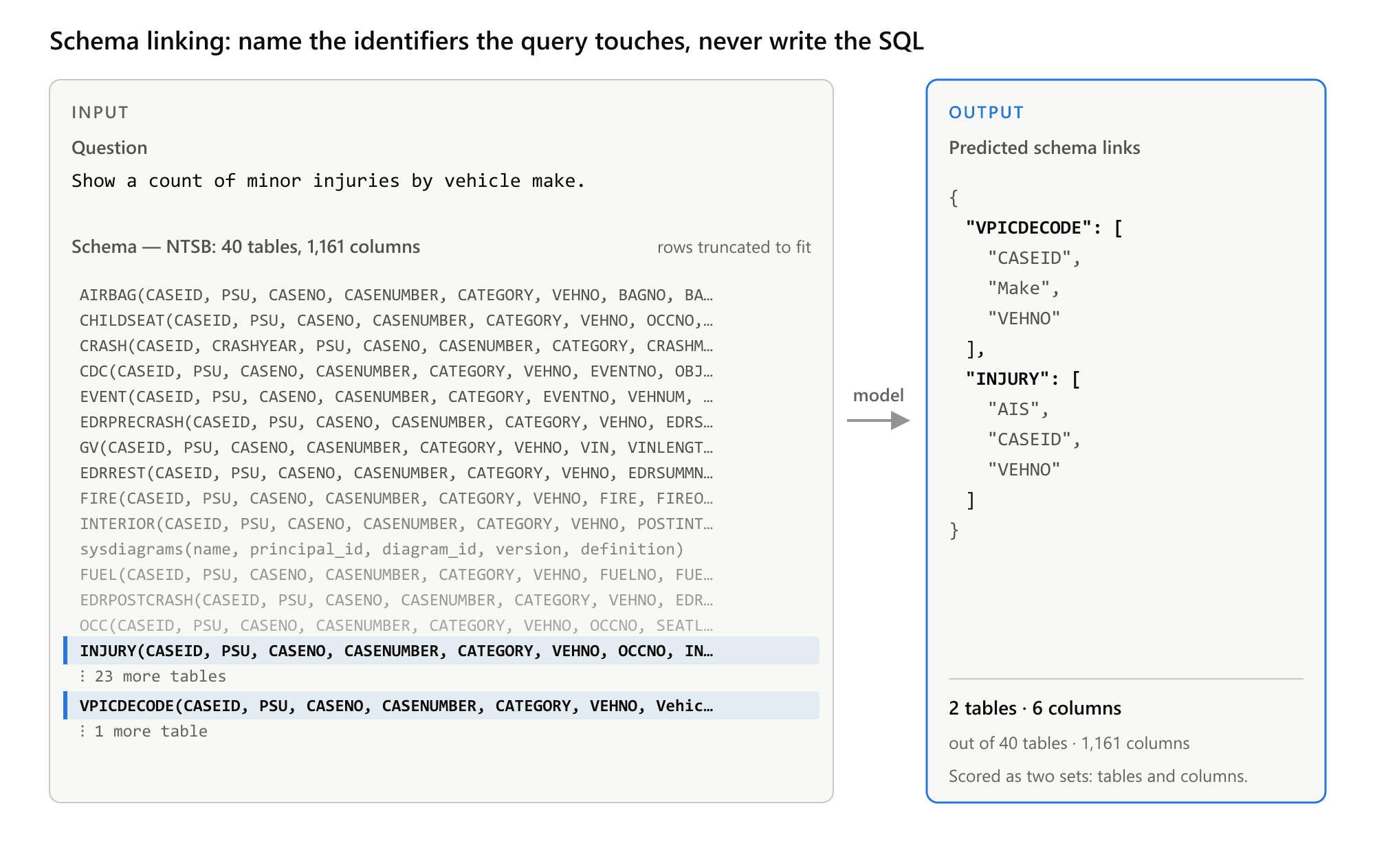
Figure 1. Schema Linking. The model receives the question and full schema as text, then returns only the tables and columns the SQL would reference. In this example, 40 tables and 1,161 columns reach the model; 2 tables are the answer. It never writes SQL.

Closed-Model APIs Set the Quality Bar

We ran 7 proprietary models through identical prompts and grader—$52.34 of live spend across 2,828 calls. Each is scored at its own best prompt configuration, since for several of them zero-shot beats few-shot on both quality and cost. The results are illustrated in Figure 2.

The quality metric is a composite score: precision, recall, and F1 at both the table and column level, averaged with equal weight across all queries.

The proprietary models set a high ceiling, with GPT-5.5, Gemini 3.1 Pro preview, and Claude Fable 5 all landing between 0.912 and 0.917. However, costs range so dramatically across these models that the cost axis is presented on a logarithmic scale.

Gemini models strictly dominate their Claude counterparts by being both cheaper and more accurate (Flash over Haiku; Pro over Opus and Fable). The Pareto frontier has three points:

• Gemini 2.5 Flash: 0.840 at $876 per million queries

• Gemini 3.1 Pro preview: 0.916 at $5,844

• GPT-5.5: 0.917 at $24,350

Going from Flash to GPT-5.5 buys 0.077 more quality for 28× the cost.

For context: returning every table and column scores 0.367 (perfect recall, weak precision), and random guessing just 0.021.

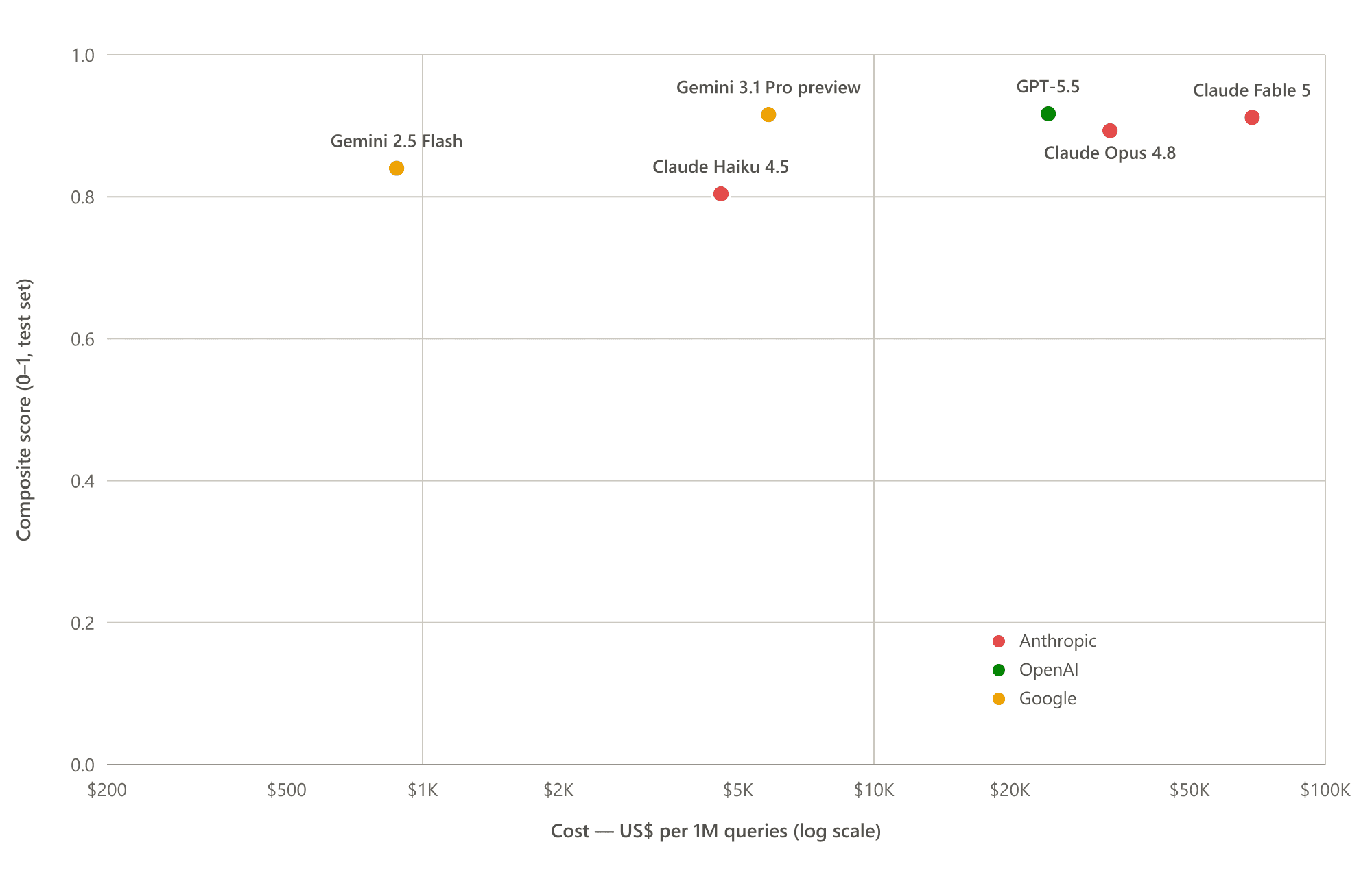
Figure 2. Cost against accuracy. The cost-quality spread of the proprietary models. Each model is shown at its own best-accuracy prompt configuration. Gemini models strictly dominate their Claude counterparts by being both cheaper and more accurate (Flash over Haiku; Pro over Opus and Fable).

The Open SLM Candidates

Against that bar we line up open, self-hostable SLMs. Our set of four instruct checkpoints probes two axes that matter here—code pretraining vs. general tuning, and small vs. larger size: a code-pretrained 1.5B (Qwen2.5-Coder-1.5B-Instruct), a general instruct 1.5B, a SmolLM2, and a 7B (see Table 1).

The code-pretrained 1.5B is our primary baseline. Untuned and zero-shot, it scores a dismal 0.351—worse than a script that just returns everything—and emits invalid JSON on 59.4% of questions, so a lenient parser has to rescue most answers before grading.

The RapidFire AI Experiment

For fine-tuning, we focus on three major design choices—base model, schema serialization, and LoRA rank. We swept all of them via a simple grid search: 4 × 2 × 2 = 16 configurations, one recipe, one seed, winner picked on validation (never the held-out test). Note that this is only a small, initial experiment by AI practice standards.

We ran SFT with RapidFire AI, our open-source experiment framework. It automatically splits all 16 runs across just 2 A100 GPUs and trains them concurrently with its “hyperparallel” execution scheme. Even when 4 SmolLM2 runs hit memory limits, the other 12 kept going untouched. Including the relaunch for SmolLM2, the sweep took 2.97 GPU-hours and 3 hours, 29 minutes of wall time.

All 16 configurations trained together on a 2-GPU box—no job queue, no babysitting runs one at a time.

What SFT Changed

Fine-tuning that 1.5B on the 301 examples (a LoRA adapter) moves it from 0.351 to 0.705 and lifts strict JSON validity from 40.6% to 100%. SFT won’t make a 1.5B a frontier model—but it roughly doubles the score and makes every response parseable.

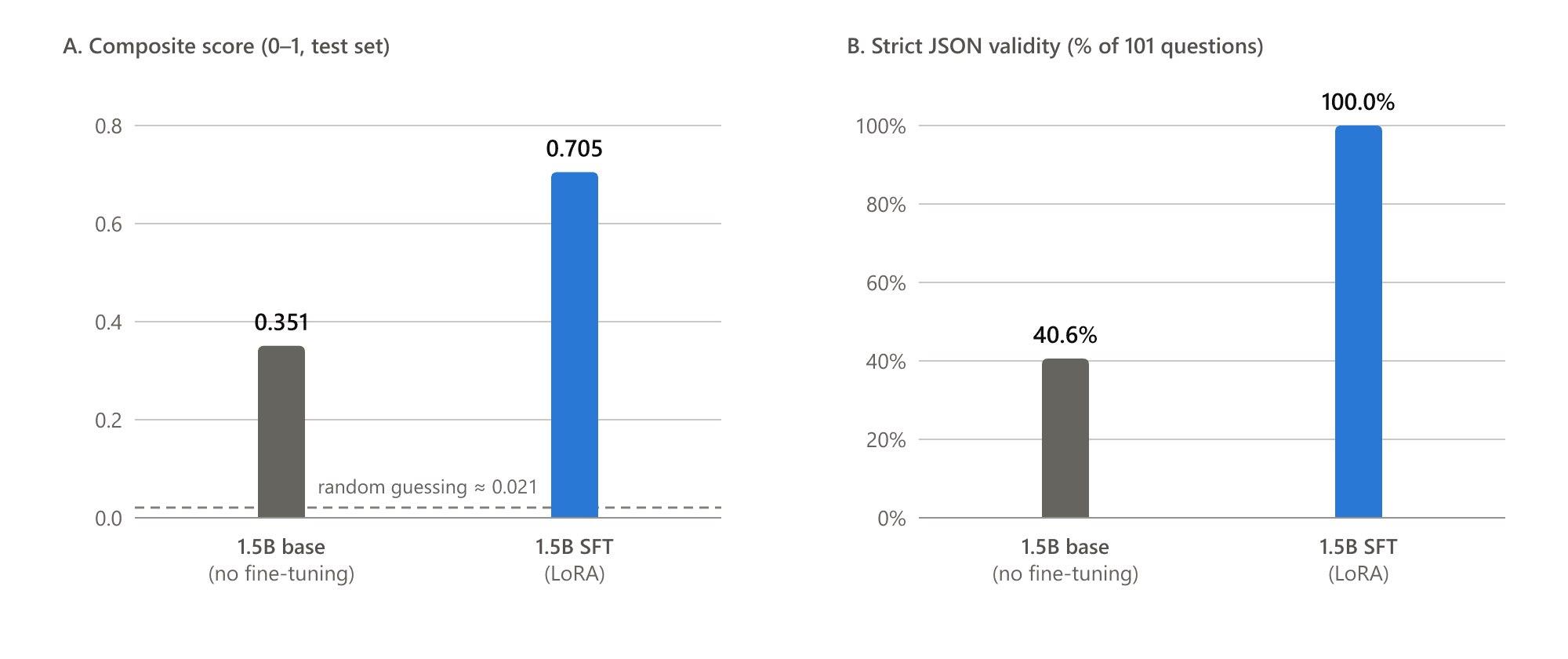
Figure 3. Fine-tuning the same 1.5B base model on 301 examples raises both composite score and strict JSON validity. The comparison uses the same prompts and grader. Both panels are zero-based and separate because score and parse rate are different quantities.

Across the sweep, we watched the same metric for all 16 configurations as they trained.

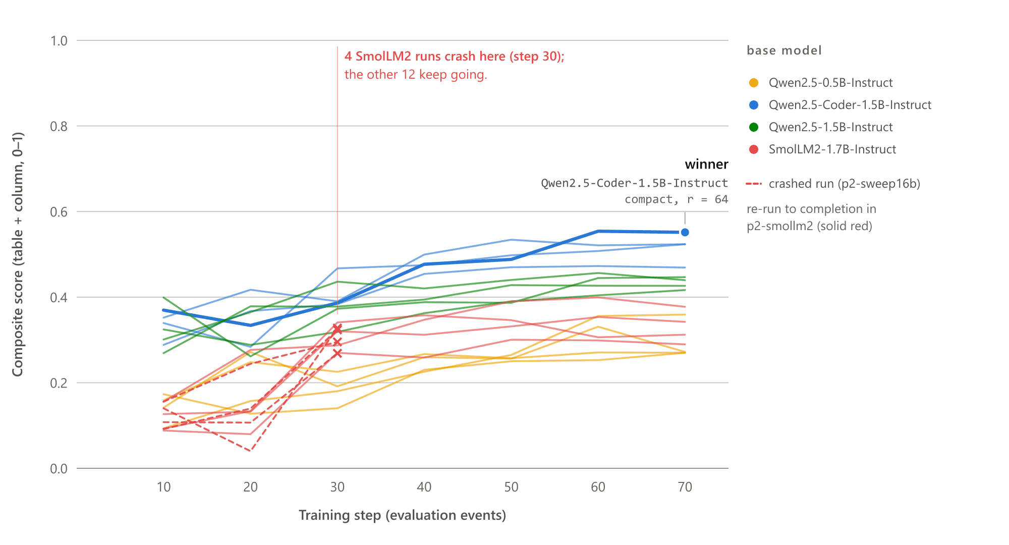
Figure 4. The y-axis is the composite schema-linking score: 0.5 × mean(table precision, recall, F1) + 0.5 × mean(column precision, recall, F1), averaged across the curve-evaluation questions. Unlike loss, this generation-based metric measures whether a model names the correct tables and columns. The curves are re-plotted from exported results; truncated SmolLM2 curves indicate runs that exhausted memory.

Only one axis—the base model—separated the runs consistently:

• Base model: the code-pretrained 1.5B beat the general instruct 1.5B in all 4 matched cells, averaging +0.044.

• LoRA rank: rank 64 helped in 7 of 8 pairs, averaging +0.033.

• Serialization: compact averaged +0.025 and won 6 of 8 pairs, but lost in the winning model’s rank-16 pair.

We picked compact serialization anyway—it’s ~46% shorter, not because it scored higher.

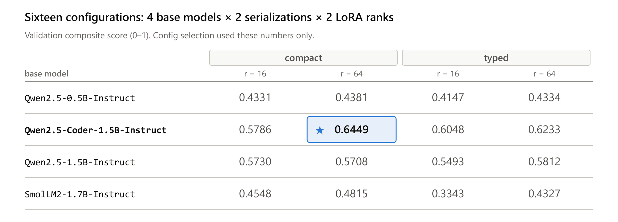
Table 1. Validation composite scores used for configuration selection; the highlighted cell is the shipped winner. Compact serialization was chosen for being shorter, not because it showed a consistent score advantage. Each configuration was trained once. Repeated runs are needed to confirm that these differences are reliable; the SmolLM2 values come from the rerun.

Comparing SLMs and Closed-Model APIs

The comparison adds two SFT points—the 1.5B and 7B. The 1.5B reaches 0.705 (about 77% of the best proprietary score) and the 7B 0.738, against the closest proprietary model, GPT-5.4-mini, at 0.765 and $2,075 per million.

The 7B trails the nearest frontier API by just 0.027 in quality—at 2.8× lower serving cost ($736 vs. $2,075 per million).

At 60% utilization, the 1.5B serves a million queries for $419.56—about 58× cheaper than GPT-5.5. The fairer benchmark is Gemini 2.5 Flash: the SLM is 2.1× cheaper but 0.135 less accurate.

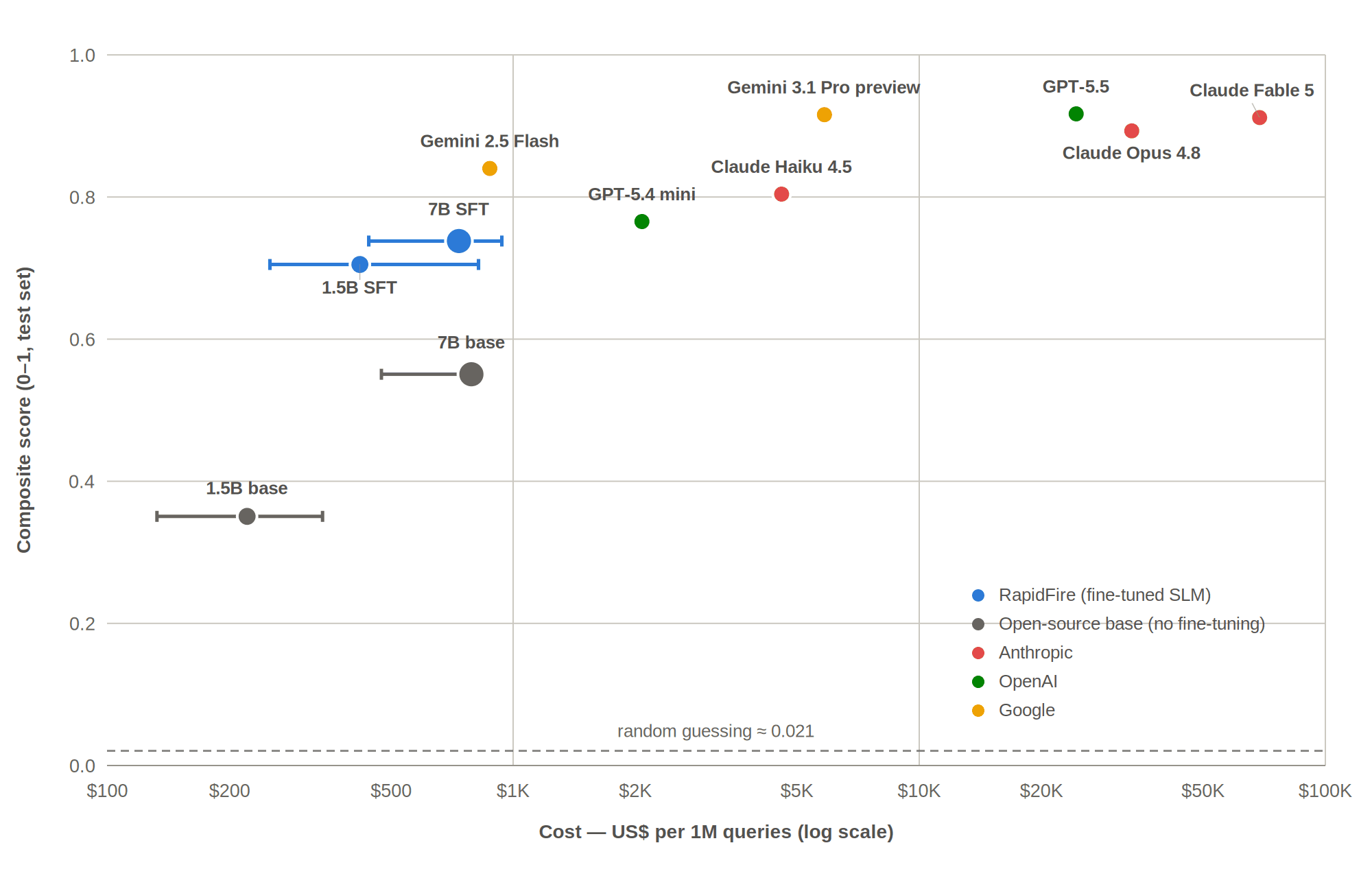
Figure 5. Cost against Composite Score. Proprietary and zero-shot SFT models are compared on composite score and cost per million queries. Dot area scales with parameter count; each SFT whisker spans saturated-GPU to batch-1 serving cost. API costs are metered, while SFT markers use amortized GPU cost at 60% utilization and shift with server utilization.

Takeaways

Frontier closed-model APIs still own out-of-the-box quality, and raw SLMs can’t touch them. But one round of SFT rewrites the math—pulling an open SLM to within 0.03 of GPT-5.4-mini. Four major takeaways:

• Focused SFT punches above its weight. 16 configs in just 3.5 hours and ~$7.52 of compute still roughly doubled the 1.5B’s score; more of both would likely push the Pareto frontier further to better match the closed models.

• Hyperparallel infrastructure made it practical. RapidFire AI trained all 16 configs at once on a single 2-GPU machine, turning what used to require a large cluster-scale search into one afternoon on modest hardware.

• Inference serving economics hinges on utilization. An SLM is far cheaper under heavy load but can lose on cost to an API at low volume. So, running SLMs at scale means investing in efficient inference serving—self-hosted or via a compliant vendor.

• The real cost of SFT for SLMs is expertise, not GPUs. Calling an API takes almost no ML engineering, but SFT takes someone who can configure and run the experiments—exactly the gap tools like RapidFire AI now close.

Reliable SFT is key for cost-efficient high-quality task-specific AI, and tooling such as RapidFire AI unlocks those options for enterprises without needing a big AI engineering team or a runaway GPU bill.

Ready to try it?

• RapidFire AI on Colab: Get Started with Fine-Tuning

• RapidFire AI on Colab: Get Started with RAG Optimization

• Code on GitHub

• Documentation